
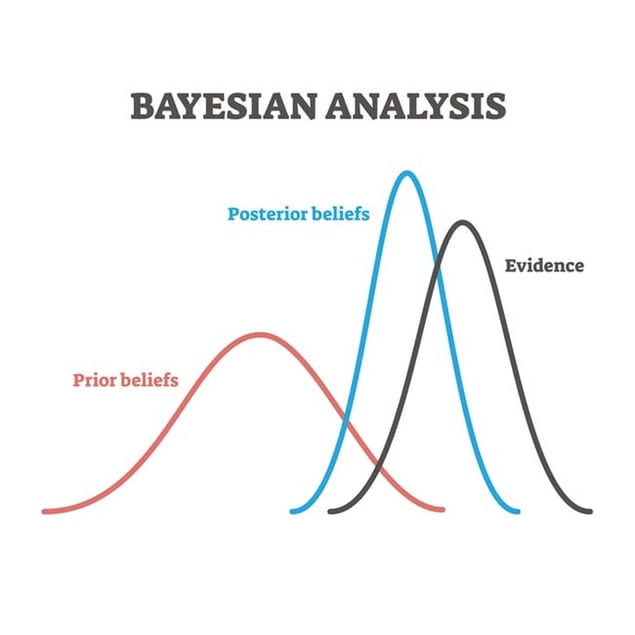
Bayesian inference is a statistical method used to update a prior belief based on new evidence, an extremely useful technique with innumerable applications. Uncertainty about probabilities that are hard to quantify is one of the challenges of Bayesian inference, but there is a solution that is exciting for its cross-disciplinary origins and the elegant chain of ideas of which it is composed.
If you’re a statistician or a data scientist you probably know the basics of Bayesian inference. If you’re just learning, the mathematical idea is to update the probability of some set of parameters based on measured data. The so-called posterior belief – the updated probability – can be defined as the likelihood of observing the new data multiplied by the prior belief and divided by the overall probability of observing model data, where the prior belief is marginalized. This gets written as there following formula, where θ is the prior belief and data is the new evidence:
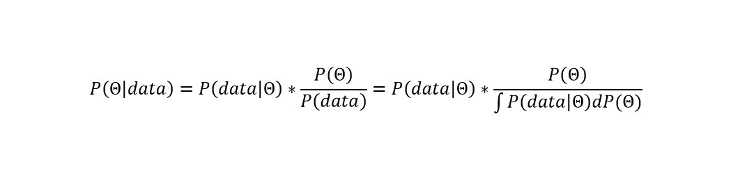
Equation 1
To make it concrete, imagine a kid who gets dessert after dinner 4 of 7 days per week. That's P(θ), the prior belief. Of the nights she gets dessert, she ate her entire dinner 2 of 4 nights. That's P(data|θ), the new evidence. But she eats her entire dinner 3 of 7 nights per week. That's P(data), the new evidence with the prior belief marginalized. So, if we execute the formula, the posterior belief is (4/7 * 2/4) / 3/7, and if the little girl finishes her dinner she has a 2/3 likelhood of getting dessert. (The injustice!)
One thing that makes Bayesian inference hard is that more often than not the integral in the denominator, also known as the normalizing constant, doesn't have a closed analytic form. It has to be numerically approximated, and it’s hard to do so. You’re estimating the probability of observing something in theory, without any evidence.
This is where the exploit of some techniques developed in very different fields comes in: Markov Chains, Monte Carlo Methods, and the Metropolis-Hastings algorithm.
Markov Chains are a very popular device for modeling stochastic – random – processes in numerous fields. The basic idea is that you can model a random process using a transition matrix where the process transitions from one state to another in some state space over time. The transition matrix lays out the probabilities for these state transitions with the transitions being memoryless i.e., the probability of transitioning from one state to another depends only on the state the process is transitioning from (and not the sequence of states the process took to get to that state). The impact of this is that as the chain evolves over a long enough period of transitions, irrespective of the initial state the process started from, the distribution over the underlying states settles into a stationary distribution. In it's simples form it is represented in this formula, where π is the stationary distribution and Τ is the transition matrix of probabilities.
 Equation 2
Monte Carlo methods are widely applied in various fields as well. These methods allow one to approximate the expectation of a function of a random variable using the sample average of the function evaluated at samples drawn from the underlying probability distribution. Ν is the number of samples drawn from the probability distribution, Ρ:

Equation 3
It turns out, under some very general assumptions, that for every probability distribution there exists a Markov chain with that distribution as its stationary distribution. So what if we were to assume that our hard to compute posterior belief (which is a conditional probability distribution) is the stationary distribution of some (unknown) Markov Chain? If we could invert a Markov Chain i.e., yield samples from the chain given its stationary distribution and assume the stationary distribution is our posterior, then we have a “magical” way of sampling the posterior without having a closed form for it! The Metropolis-Hastings algorithm allows us to do just that. It allows us to automatically compute the transition matrix in Equation 1 given only the easy to compute numerator terms in Equation 2. The normalizing constant is not needed. As the algorithm iterates, its iterations yield samples from our posterior.
How does that help? As we sample the posterior, we can easily do either of the following:
- Estimate the posterior probability, e.g.: by constructing a sample histogram using these samples. This histogram approximates the density of the underlying probability distribution.
- Compute Bayesian predictions. Use the Monte Carlo rule from Equation 2 to approximate the expected value of a prediction for a new data point over the entire model parameter space by the sample average of the predictions computed at parameter values sampled from the posterior.
The Monte Carlo methods were developed in the 1940s in Los Alamos during World War II by a team of physicists working on the Manhattan Project. The Metropolis-Hastings algorithm was subsequently developed in the 1950s at Los Alamos by Nicolas Metropolis working on many-body problems in statistical mechanics and later generalized by W. Hastings in 1970s. With the emergence of computing power in the 1980s, there was a rapid surge in the decade to follow in the application of these algorithms to problems in fields ranging from computational biology to finance and business that had proven intractable with other mechanisms. Decades-old ideas originally developed in one field have served to make contributions in different areas many years later - evolving Bayesian inference via exaptation.

Comments